Original Projection, Cartesian trapezoidal methods, and earlier Turns formulations retain their own definitions and scope. They are not interchangeable specifications.
Evidence
Geometric accuracy, floating-point stability, computational performance, and originality are separate questions. See Results and the benchmark protocol for their status.
Generative Radial Geometry: Radius, Rotation, and Arc Length
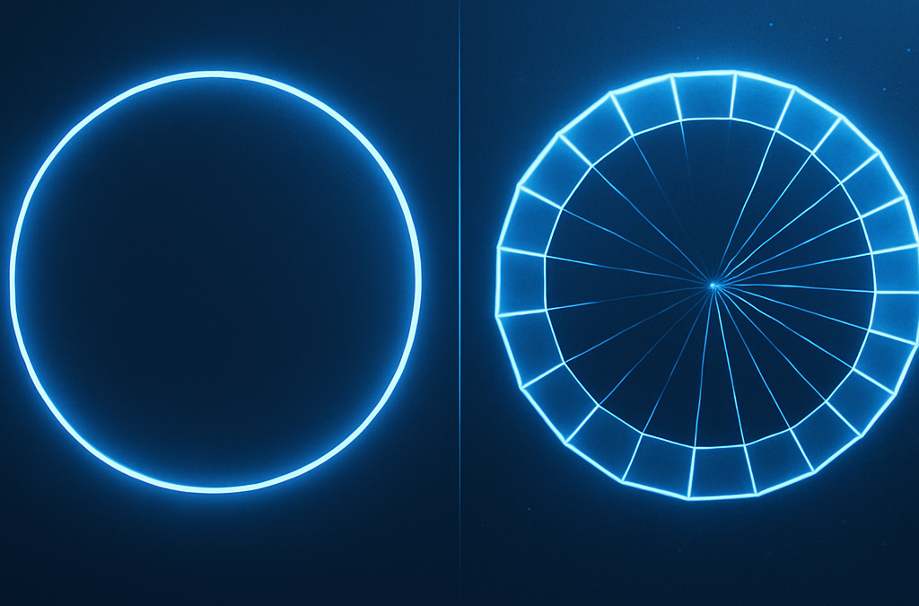
Generative Radial Geometry (GRG) provides a discrete, π-free, constructive method to generate circles, spheres, and related shapes. Instead of assuming π and continuous formulas, GRG builds geometry from radial divisions, summing chords and trapezoids. This creates a radically different perspective compared to the classical approach. Angles are expressed as fractions of the turn ($u\in[0,1)$).
Why GRG Matters
Classical geometry relies on π and continuous trigonometric functions. GRG, in contrast, is digital-native: it works with finite steps, exact points on the circumference, and simple arithmetic operations. This makes it both conceptually new and computationally efficient.
Core Comparison
The table below highlights the key differences between the two approaches.
Aspect
Classical Approach
Generative Radial Geometry (GRG)
Definition of angle
Radians \((s=r\theta)\) with \(\pi\).
Angle = discrete fraction \(k/N\) of the turn \((u\in[0,1))\), generated internally.
Mathematical tools
Trigonometry, sine/cosine, continuous integrals.
Finite sums of chords and trapezoids; additions and square roots.
Exact by construction on generated radial sets \((x^2+y^2=R^2)\).
Lengths and areas
Closed forms: \(s=r\theta\), \(A=\pi R^2\).
Generated sums: \(L=\sum \ell_i\), \(A=\sum A_i\); \(\pi\) emerges as a limit.
Local error
None in theory, but depends on \(\pi\)/trig numeric precision.
Error only from finite sums; boundary points remain exact.
Extension to 3D
New formulas needed (e.g., \(V=\tfrac{4}{3}\pi R^3\)).
One constructive scheme extends to surfaces and volumes.
Computational efficiency
Expensive trig; slower on low-level hardware.
Roots + sums; friendly to SIMD/GPU and embedded devices.
Concept of \(\pi\)
\(\pi\) assumed a priori.
\(\pi\) appears from the discrete generative process.
Conceptual view
Geometry as a static entity to be measured.
Geometry as an internal, generative process.
Three GRG Modes
On this page we use three operational modes. Two are Cartesian and compute area on a quarter (by symmetry). One is radial and computes circumference on the full turn.
Mode
Target
Partition
Element
Estimate
Formula (sketch)
Notes
Δx Trapezoidal (Cartesian)
Area
Quarter, \(x_i=i\,\Delta x\), \(\Delta x=R/N\)
Trapezoids between heights \(h_i=\sqrt{\,R^2-x_i^2\,}\)
Lower (under-tiling)
\(A_Q \approx (\Delta x/2)\sum(h_i+h_{i+1})\); total area \(=4\,A_Q\)
Monotone ↑ with \(N\)
Projection Corridor (Cartesian)
Area
Quarter, same \(\Delta x\)
Riemann-like bars at right / midpoint
Lower/Upper (squeezing)
\(A_Q^{\downarrow}=\Delta x\sum h_i\), \(A_Q^{\uparrow}=\Delta x\sum h_{i+\tfrac12}\); total \(=4\times\)
Certified bounds
Chord-Sum at \(\Delta u\) (Radial)
Circumference
Full turn, \(\Delta u=1/N\)
Chords between consecutive radial points
Lower (inscribed polygon)
\(L \approx N\,R\,\sqrt{\,2-2\,c(1/N)\,}\)
No quarter; defined on the whole circle
Note on “quarters”. The quarter is used only for the Cartesian area modes (by symmetry). For circumference we operate on the full turn (radial partition), so “quarters” are not meaningful there.
Further Evaluations & Options
Certified area bounds. The corridor (right vs midpoint) yields lower/upper bounds that squeeze the exact area as \(N\) grows.
Stronger circumference bracketing. Pair the inscribed chord-sum (lower) with a circumscribed tangent-sum (upper) to bound the true length.
Adaptive refinement. Increase \(N\) only where variation is largest (near endpoints for Cartesian area; uniform \(\Delta u\) usually suffices for chords).
Hybrid pipelines. Use circumference from chords to cross-check the discrete derivative of area w.r.t. \(R\).
3D extension. The same logic generalizes to spherical belts (length) and frusta/patch sums (area/volume) with discrete radial partitions.
Hardware efficiency. All modes need only sums and square roots → ideal for embedded, SIMD, and GPU kernels.
Conclusions
Classical geometry excels in closed-form elegance. GRG complements it with a digital-native, constructive view: exact boundary points, sums that converge without assuming π, and a single scheme that scales from 2D to 3D. Here we use three GRG modes—two Cartesian for area on a quarter, one radial for circumference on the full turn—unlocking certified bounds, adaptive strategies, and hardware-friendly implementations.
Generative Radial Geometry for Chemistry: From Conformers to MOFs and Solvent Shells
Angles in turns. We sample directions with turns \(u\in[0,1)\) at \(\Delta u=1/N\) (full turn). This keeps angular steps digital-native and π-free.
Generative Radial Geometry (GRG) offers a center-out way to construct and search chemical structures. By organizing atoms, coordination sites, pores, or solvent molecules in radial shells with controlled distances and angles, GRG cuts down the combinatorial explosion and makes 3D models that are physically plausible and immediately ready for simulation.
Where GRG helps in chemistry
Molecule modeling & design: targeted conformer generation around rings and chiral centers; pre-screening of virtual libraries to propose sterically sensible radial scaffolds.
Crystallography & solids: crystal packing via radial neighborhoods of a repeat unit; localized models of defects and vacancies.
Molecular dynamics: fast computation of radial distribution functions (RDF) and balanced initialization of solvents/ions around a solute.
Porous materials (MOF/COF): radial placement of metal nodes around linkers; geometric control of free radii to tune pore accessibility.
Supramolecular self-assembly: prediction of micelles/liposomes and core–shell architectures by concentric, composition-aware layers.
Drug design & docking: radial abstractions of binding pockets and “radial grids” of electrostatic potential to guide polar/apolar moieties.
GRG Modes & Selection (Chemistry). We use three base modes:
Δx Trapezoidal (area-like sums on a quarter, lower estimate),
Projection Corridor (paired lower/upper bounds on a quarter),
and Chord-Sum at Δu (loops on the full turn, lower; pair with tangent-sum for an upper bound).
In 3D they extend naturally to spherical shells/belts/frusta.
Uniform directions \(u\in[0,1)\) for conformers/solvent placement.
Pore apertures & ring tiling in MOFs/COFs; angular RDF slices.
Picker by task. Need speed → Trapezoid; need guarantees/threshold radii → Corridor; need angular uniformity/phase on rings → Chord-Sum (± tangent-sum); volumetrics → shell/belt extensions.
Core GRG idea for chemical systems
Place partners within radial bounds and enforce angular/steric constraints; then score candidates and iterate. Typical constraints:
GRG modes: Use Trapezoid to accumulate RDF shell counts quickly; switch to Corridor for certified bounds on coordination \(N(R)=4\pi\rho\!\int_0^R\!g(r)\,r^2dr\); use Chord-Sum at \(\Delta u=1/N\) to ensure uniform angular sampling when RDF is evaluated over directional sectors.
Worked examples
1) Conformer generation around a chiral center
Goal: explore the spatial arrangements around a chiral carbon and select the most stable isomer.
Define the chiral center C and the four substituents (A, B, C, D).
Choose distance bounds for C–X: e.g., 1.45–1.55 Å.
Partition the interval into k concentric shells (e.g., 5).
On each shell, sample directions with turns \(u\in[0,1)\) at \(\Delta u=1/N\), enforcing tetrahedral angles ≈\(109.5^\circ\) and min separations.
Score with a light force field (e.g., UFF) and retain the lowest-energy 10 conformers.
GRG modes:Chord-Sum (full turn, turns \(u\)) for uniform angular sampling and ring-wise sterics; Trapezoid to tally shell feasibility quickly; Corridor to certify bounds on steric/energy scores over shells before QM refinement.
2) Crystal packing of a simple MOF
Goal: arrange metal nodes and organic linkers in a cubic unit cell using radial symmetry.
Place a metal node M (e.g., Zn2+) at the cell center; four linkers L at the corners of a radial tetrahedron.
Set coordination bounds (e.g., M–O = 1.9–2.2 Å).
For each L site, sample positions on a spherical shell about M, keeping \(\angle\text{L–M–L}\approx 109.5^\circ\).
Tile the cell periodically with vectors \((a,0,0)\), \((0,a,0)\), \((0,0,a)\).
Run a short geometry minimization (e.g., Powell) to relieve strain.
GRG modes:Chord-Sum for ring apertures and angular registry of linkers (periodic tiling over full turn); Trapezoid for cross-sectional pore area scans (quarter ×4); Corridor to bound pore-limiting/free-sphere radii derived from those scans.
3) Solvent bubble for MD around a solute
Goal: generate a balanced water sphere around a charged solute without overcrowding.
Locate the solute center of mass and choose \(R_1\) (solute + first shell) and \(R_2\) (outer boundary).
Split \([R_1,R_2]\) into \(N\) shells (typically 3–5).
For each shell, place water molecules by sampling directions uniformly with turns \(u\) and \(\Delta u=1/N\); set distances \(r\) within that shell and enforce \(d_{\min}(\mathrm{O}, \text{solute}) \ge 2.5\ \text{Å}\).
Assign water orientations (H–O–H) with small random perturbations.
Export to PDB and run a short heating/minimization to relax the sphere.
GRG modes:Chord-Sum for uniform angular placement/orientations; Trapezoid for quick shell occupancy and radial density; Corridor to bracket hydration numbers \(N(R)\) and to stop when bounds meet your tolerance.
4) Docking on radial electrostatic grids (quick setup)
Goal: approximate binding pocket neighborhoods with radial shells and guide pose sampling.
Center a pocket reference and define shells \([r_k,r_{k+1}]\) plus ring samples at turns \(u_j=j/N\).
Precompute coarse electrostatic potential on these cells; score ligand fragments by shell and ring.
Promote top cells to fine sampling; enforce sterics and ring-wise clashes; export poses to your docking engine.
GRG modes:Chord-Sum for ring coverage of orientations; Trapezoid to roll up cell scores radially; Corridor to keep upper/lower envelopes on pocket accessibility/energy as you refine.
From generation to computation
Search space reduction: symmetries and radial bounds focus the exploration on chemically sensible regions.
3D realism with control: enforce minimum/maximum inter-center distances and angles while sampling.
Drop-in to pipelines: GRG output meshes with QM, MD, and docking workflows (e.g., UFF pre-screen → PDB export → MD heating → production run).
GRG modes (pipeline): Use Trapezoid during fast scans; switch to Corridor to certify thresholds (coordination/hydration/pore radii); validate angular uniformity/perimeters with Chord-Sum (± tangent-sum) before committing to costly runs.
Conclusion
Across molecular design, crystal engineering, porous frameworks, self-assembly, and simulation setup, GRG brings a clear center-out logic: define radial bounds, discretize into shells, generate angles under constraints, and score. Choosing among Δx Trapezoidal, Projection Corridor, and Chord-Sum at Δu—or combining them—yields fast baselines, certified bounds, and robust angular control for meaningful chemistry.
RDF & Coordination via GRG Corridor — bounds on N(R) and Rn
Definitions. With bulk number density \(\rho\) and radial distribution \(g(r)\), the
coordination number inside radius \(R\) is
$$
N(R)=4\pi\rho\int_0^{R} g(r)\,r^2\,dr.
$$
Discrete GRG shells. Choose radii \(0=r_0turns \(u\in[0,1)\)) and use min/max over the sector.
where \(g_k^{\min},g_k^{\max}\in\{g_k^{\mathrm{in}},g_k^{\mathrm{out}}\}\) for smooth/monotone segments, or the
angular min/max in that shell otherwise. Always \(N^{\downarrow}(R)\le N(R)\le N^{\uparrow}(R)\).
Bracketing a coordination radius. For a target coordination \(n\) (e.g., “first shell”):
\(R_{n}^{-}=\min\{R:\,N^{\uparrow}(R)\ge n\}\) is a lower bound of the true \(R_n\).
\(R_{n}^{+}=\min\{R:\,N^{\downarrow}(R)\ge n\}\) is an upper bound of the true \(R_n\).
Refine by halving shell width \(\Delta r\) near the bracket or by bisecting within the shell until
\(R_{n}^{+}-R_{n}^{-}\le\) tolerance.
Method picker. Isotropic liquids: use shells only (fast). Structured/anisotropic systems or near interfaces:
split shells into polar cells; sample azimuth with Chord-Sum (\(\Delta u=1/N\)) to keep directional coverage,
then apply the corridor per cell. Use Trapezoid for quick scans of \(N(R)\); switch to Corridor when you need guarantees.
Practical notes. Use \(\Delta r\) small enough to resolve the first peak of \(g(r)\)
(typ. 0.02–0.05 nm); respect PBC and the minimum-image convention (limit \(R\le L/2\) in a cubic box).
For noisy \(g(r)\), smooth lightly after computing corridor bounds, not before.
Generative Radial Geometry for Optics: From Aspheres to Metasurfaces
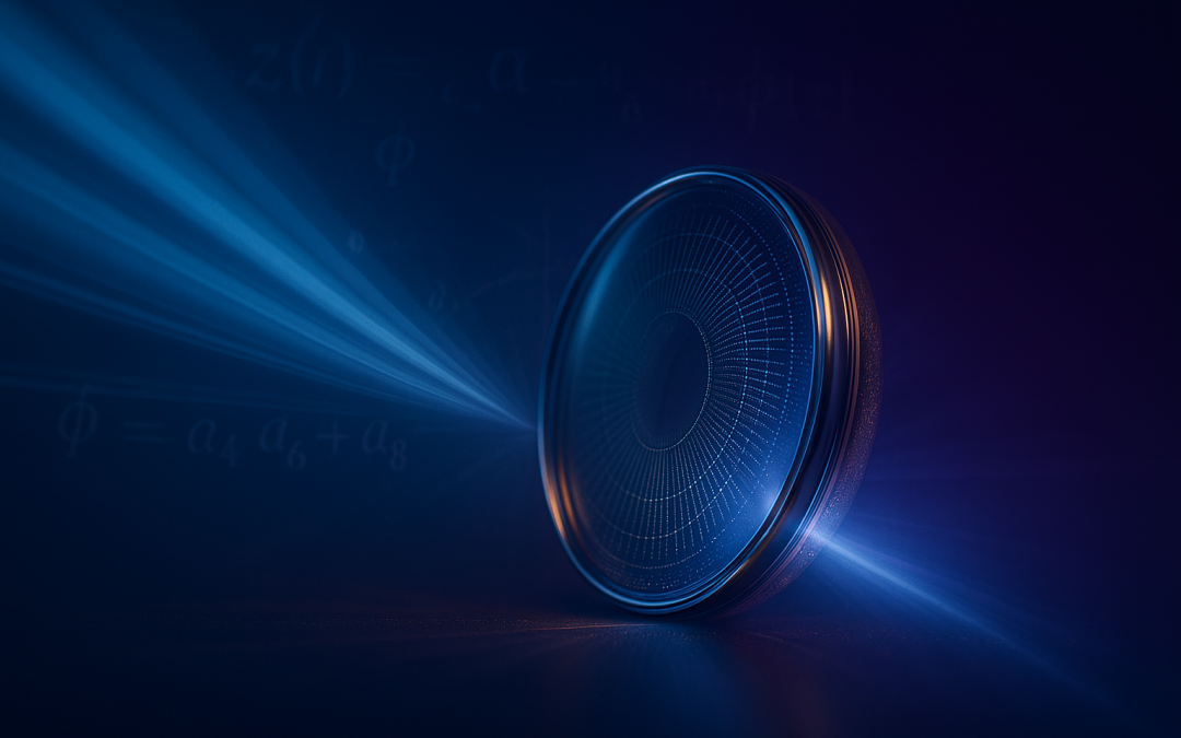
Generative Radial Geometry (GRG) treats optical elements as radially generated structures optimized from the center outward. This viewpoint enables targeted aberration correction, compact/lightweight systems, and fast iteration via simulation—spanning refractive aspheres, GRIN profiles, diffractive zone plates, and radially programmed metasurfaces.
What GRG means in optics
In GRG, a surface or refractive-index profile is parameterized radially and then optimized against a merit function (e.g., wavefront error, Strehl, or MTF) over the full pupil. Rather than restricting to a low-order conic/asphere, GRG explores richer radial degrees of freedom that better align the phase over wide apertures and fields.
GRG Modes & Selection for Optics. We use three base modes: Δx Trapezoidal (fast area-like radial sums, lower estimate), Projection Corridor (paired lower/upper area bounds via right/midpoint sampling), and Chord-Sum at Δu (circumference/loops on the full turn, lower; pair with tangent-sum for an upper bound). In optics they map to pupil integrals (energy/WFE), certified bounds on merit terms, and phase/loop controls on rings/zones.
Encircled energy, WFE/OPD RMS, throughput vs radius.
Baseline fast integration in design loops.
Projection Corridor
Target: same as above • Estimate: lower & upper (certified)
Bounds for energy, WFE, Strehl/MTF contributions.
Use to stop/refine when gap ≤ tolerance.
Chord-Sum at Δu (Radial)
Target: loops on rings (full turn) • Estimate: lower (pair with tangent-sum ↑)
Zone edges, phase wraps (2π), vortex/Bessel rings.
Perimeter/phase uniformity & ring tiling quality.
Picker by task. Quick merit updates → Trapezoid; need guarantees → Corridor; ring/zone phase & perimeter → Chord-Sum (± tangent-sum); 3D volume/weight/thermal → shell/frusta extensions.
Why GRG improves optical design
Targeted aberration correction: spherical aberration, coma, and astigmatism can be minimized across large apertures by flattening phase error over the beam.
Compact, lightweight systems: high-performance single elements can replace multi-lens groups; GRG also supports radial GRIN to combine focus and correction in one body.
Advanced diffractive elements: optimized radial zone partitioning for resolution, efficiency, and robustness—supporting multi-order/multi-focal designs.
Metasurfaces & LIDAR: radial placement/shaping of nano-scatterers for phase/amplitude control (beam shaping, Bessel/vortex), wide-FOV collimation, compact 360° sensing.
Rapid simulation-to-prototype: GRG loops tightly with FEM/FDTD engines to explore candidate radial profiles quickly.
Design workflow (radial parametrization → merit function → solver)
A typical GRG workflow parameterizes the sag or index as a radial series; samples the pupil; defines a merit function over wavefront or image metrics; and solves for the radial coefficients (often via linearization around a base conic).
Radial surface model
We model the sag z(r) as a base conic plus a radial polynomial tail:
$$
M
\begin{pmatrix}
a_{4}\\[2pt]
a_{6}\\[2pt]
a_{8}
\end{pmatrix}
\;=\;
b.
$$
GRG modes: Use Trapezoid for fast radial contributions to WFE/energy; switch to Corridor when you need a guaranteed bound on residuals; use Chord-Sum on rings to enforce phase consistency (2π wraps) and to check zone/perimeter uniformity; add tangent-sum to bracket loop metrics.
Worked example: aspheric–radial singlet at λ = 550 nm
For a collimated beam at λ=550 nm focused to f=100 mm with D=25 mm, take a base paraboloid (k=–1) with curvature c=0.010 mm⁻¹ (R=100 mm). Solving the linearized system yields:
With these coefficients, the residual wavefront error across the pupil falls below λ/20 and the MTF at 50 lp/mm improves by ~30% relative to the spherical counterpart:
GRG modes: Trapezoid for quick MTF/Strehl-related radial sums; Corridor to certify WFE/energy targets before freezing coefficients; Chord-Sum (+ tangent-sum) to monitor ring-wise phase/perimeter and edge artifacts.
Diffractive optics and zone plates
GRG optimizes the radial subdivision and phase steps of diffractive optical elements (DOEs) to jointly maximize resolution, first-order efficiency, and fabrication tolerance, and can be extended to multi-order/multi-focal targets.
GRG modes: Chord-Sum to place ring edges by phase advance along the circumference (2π steps, vortex charge checking); Corridor to bound first-order efficiency/EE across radii; Trapezoid for throughput and fill-factor roll-ups.
Metasurfaces and 360° sensing (LIDAR)
For metasurfaces, GRG prescribes the radial distribution and geometry of nano-scatterers (meta-atoms) to deliver the desired phase/amp profile—enabling beam shaping (Bessel, vortex), wide-FOV collimation, or compact 360° sensing modules.
GRG modes: Chord-Sum for ringwise phase conformity and azimuthal uniformity (Bessel/vortex); Corridor to bracket efficiency across pupil zones under scatterer quantization; Trapezoid for fast aggregate metrics during layout sweeps.
GRIN materials and fabrication
Beyond pure surface shaping, GRG covers radial gradient-index (GRIN) profiles co-optimized with geometry, compatible with precision 3D printing, advanced lithography, and layered deposition processes.
GRG modes: Trapezoid/Corridor for OPD and energy integrals through shells (robustness to dispersion/tolerances); Chord-Sum to verify iso-phase circles after co-optimizing n(r) + sag.
Simulation loop and time-to-prototype
A GRG toolchain linked to wave/EM solvers rapidly screens candidate radial profiles, reducing the number of physical iterations needed before fabrication.
GRG modes: Loop fast with Trapezoid; certify with Corridor (stop when the bound gap is within tolerance); validate ring/zone behavior with Chord-Sum (+ tangent-sum) before tape-out.
Practical notes: tolerances, costs, and when GRG is worth it
Tolerancing: include manufacturing/assembly error budgets in the merit function so the solved profile remains robust after polishing, litho rounding, or index dispersion.
Cost trade-offs: in commodity systems, classic low-order aspheres may stay cheaper; GRG shines when performance/weight constraints justify advanced profiles.
System impact: a single GRG element can replace a small lens group—simplifying alignment and improving thermal stability—especially with GRIN or metasurface layers.
Conclusion
GRG augments—not replaces—classical optical design. By combining Δx Trapezoidal, Projection Corridor, and Chord-Sum at Δu (with tangent-sum for upper loop bounds), you get fast merit updates, certified guarantees, and precise ring/zone control across refractive, diffractive, GRIN, and metasurface optics.
Encircled Energy (EE) via GRG Corridor — bounds on Rτ
Definition. For a pupil-normalized PSF intensity \(I\), the encircled energy at radius \(R\) is
where \(I_k^{\min}, I_k^{\max}\) can be chosen as \(\{I_k^{\mathrm{out}}, I_k^{\mathrm{in}}\}\) for monotone-decreasing \(I(r)\),
or via angular min/max for general PSFs. Always \(E^{\downarrow}(R)\le E(R)\le E^{\uparrow}(R)\).
Bracketing the EE radius. For a target \(\tau\) (e.g., 0.80):
\(R_{\tau}^{-}=\min\{R:\,E^{\uparrow}(R)\ge \tau\}\) is a lower bound on the true \(R_{\tau}\).
\(R_{\tau}^{+}=\min\{R:\,E^{\downarrow}(R)\ge \tau\}\) is an upper bound on the true \(R_{\tau}\).
Refine by increasing annuli (or bisect within the bracket). Stop when \(R_{\tau}^{+}-R_{\tau}^{-}\le\) tolerance.
Method picker. Axisymmetric/on-axis: use annular corridor above (fast). General PSF or field points: use GRG Projection Corridor on a quarter (area bounds), or polar cells with per-cell min/max. Use Chord-Sum (+ tangent-sum) to validate ring perimeter/phase uniformity when EE is tied to zone edges.
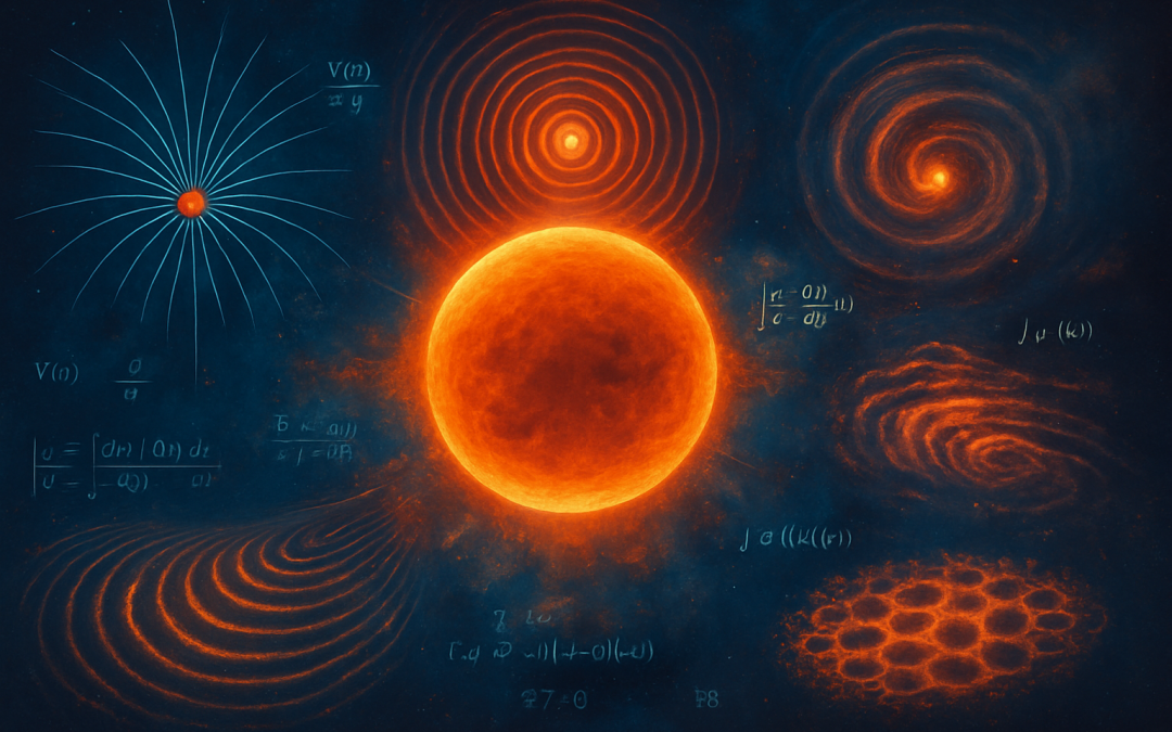
Abstract. Many physical phenomena are inherently radial: fields, waves, and potentials often depend primarily on the distance from a center. Generative Radial Geometry (GRG) provides a constructive, π-free approach to model, simulate, and visualize these systems through concentric layers and radial discretization. This article illustrates applications of GRG in major areas of physics.
GRG modes & selection. We use three base modes: Δx Trapezoidal (area on a quarter, lower bound), Projection Corridor (area bounds on a quarter, lower/upper), and Chord-Sum at Δu (circumference on the full turn, lower bound). In 3D, they extend to spherical belts/shells and frusta. Combine them as needed: corridor for certified bounds, trapezoid for speed, and chord-sums (plus tangent-sums) for tight perimeter/phase loops.
GRG Modes & Quick Picker
Δx Trapezoidal (Cartesian)
Target: area on a quarter (by symmetry); estimate: lower.
Heights \(h_i=\sqrt{R^2-x_i^2}\) with \(\Delta x=R/N\). Fast baseline integration for energy/flux cross-sections.
Projection Corridor (Cartesian)
Target: area on a quarter; estimate: lower & upper.
Right-endpoint vs midpoint bars → certified bounds and convergence checks.
Chord-Sum at Δu (Radial)
Target: circumference on the full turn; estimate: lower.
Inscribed polygon with \(\Delta u=1/N\); pair with a circumscribed tangent-sum for upper bounds.
Method picker (by task): cross-section integrals → Trapezoid/Corridor; error-bounded areas → Corridor; loop/perimeter or phase → Chord-Sum (± tangent-sum); 3D shells/belts for volumetric fields and transport.
GRG builds 3D maps of the potential and simulates test-particle trajectories in radial orbits.
Figure 1 — Radial field layers and flux lines around a central source.
GRG modes: Trapezoid for fast radial flux integrals; Corridor for bounds on energy over cross-sections; Chord-Sum for closed-loop circulation/perimeter (pair with tangent-sum for bounds).
2. Quantum Mechanics
Example A – Hydrogen atom states: The wavefunction separates into radial part \(R_{n\ell}(r)\) and angular part \(Y_{\ell m}(\theta,\varphi)\). GRG discretizes \(R_{n\ell}(r)\) on radial lattices, reconstructing 3D probability clouds.
Example B – Central harmonic oscillator:
$$
V(r)=\tfrac{1}{2}m\omega^2 r^2
$$
GRG visualizes radial energy levels and wavefunctions.
Figure 2 — Radial harmonic potential and discrete energy shells.
GRG modes: Trapezoid/Corridor for radial probability/energy integrals (with bounds); Chord-Sum for phase on circular paths or ring traps; 3D shell sums for normalization/expectation over spheres.
3. Fluid Dynamics and Plasmas
Example A – Radial plasma outflow (solar wind): Velocity \(v(r)\) and density \(\rho(r)\) vary with distance from the Sun. GRG constructs radial flow maps and shock profiles.
Example B – Accretion disk stability: Radial perturbations \(\delta\Sigma(r)\) satisfy Sturm–Liouville equations. GRG produces concentric density/pressure maps to study instabilities.
GRG modes: Corridor to bracket mass/flux through circular sections; Trapezoid for fast updates in time-stepping; Chord-Sum to track expanding wavefront perimeters.
4. Condensed Matter Physics
Example A – Metallic nanoparticle: Electronic density of states \(g(r,E)\) varies radially. GRG simulates plasmon resonances (volume vs surface modes).
GRG discretizes concentric shells to generate radial temperature solutions.
GRG modes: 3D shell/frusta extensions for volumetric integrals; Corridor for error-controlled cross-sectional energy; Trapezoid for quick area-based approximations.
GRG generates concentric pressure fields for wave propagation.
Example B – Resonances in spherical cavities: Solutions involve spherical Bessel functions \(j_\ell(kr)\). GRG maps radial nodes and mode structures.
GRG modes: Chord-Sum for wavefront loops and boundary phase; Corridor to bound average energy over sections; 3D shell sums for full energy content.
6. Nonlinear Dynamics and Pattern Formation
Example A – Radial reaction–diffusion:
$$
\begin{cases}
\partial_t u = D_u(\partial_{rr}u+\tfrac{2}{r}\partial_r u)+f(u,v),\\[6pt]
\partial_t v = D_v(\partial_{rr}v+\tfrac{2}{r}\partial_r v)+g(u,v).
\end{cases}
$$
GRG generates concentric patterns (e.g., chemical oscillations of Belousov–Zhabotinsky type).
Example B – Shock waves: Radial GRG models produce animated fronts and radial profiles of pressure and density.
GRG modes: Corridor for bounds in reactive mass/energy; Trapezoid for fast snapshots; Chord-Sum to track shock ring perimeters and speed.
Conclusion
Across physics, GRG offers a unified radial framework to generate, analyze, and visualize systems with spherical or circular symmetry. By choosing among Δx Trapezoidal, Projection Corridor, and Chord-Sum at Δu—or combining them—you can obtain fast baselines, certified bounds, and tight perimeter/phase control. In 3D, their shell/belt/frusta extensions scale the same logic to full volumetric phenomena.
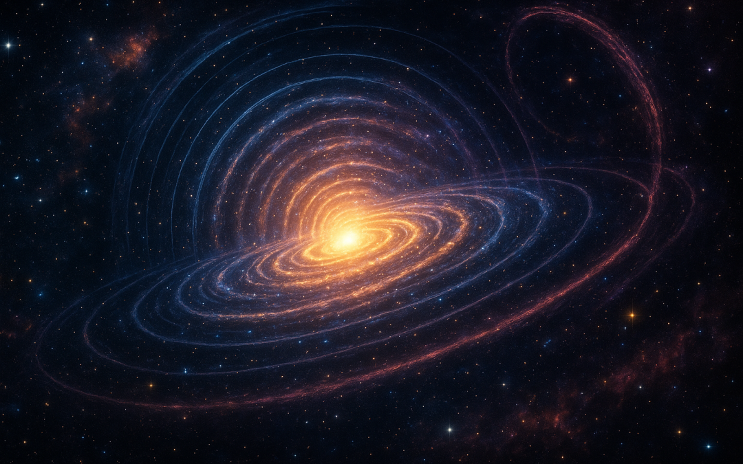
Abstract. Generative Radial Geometry (GRG) is a discrete, π-free approach that models shapes from the inside-out via radial generation. Because many cosmic phenomena are radially organized—from galactic halos to gravitational lenses—GRG offers natural, efficient tools to simulate, analyze, and visualize the universe.
GRG notation. Angles are fractions of a full turn: u∈[0,1). A turn-based logarithmic spiral is written as r = a·e^{βu}, where β controls growth per turn. This avoids π and keeps the representation digital-native.
Hero — Radial Layers with Logarithmic Arms (turn-based)
Figure 0 — Radial layers with two opposite logarithmic spiral arms r=a\,e^{\beta u}.
Radial Mapping of Stellar and Galactic Systems
Galaxies and clusters frequently exhibit radial or pseudo-radial structure. GRG models such systems as cumulative radial layers:
$$
\rho(r)=\sum_{k=1}^{N} f_k(r)
$$
This representation captures luminosity gradients and supports multi-scale “zoom” without discontinuities.
Dark Matter Distribution
Halo profiles are commonly modeled by radial functions such as the Navarro–Frenk–White (NFW) profile:
This allows continuous navigation across scales and directions without discontinuities.
Figure 3 — Rings + angular sectors for within-r queries and multi-resolution bins.
Computational Benefits
Multi-scale coherence: continuous zoom from core to periphery
Simplified algorithms in radial/turn coordinates
Natural fit for circular or spherical symmetries
Efficient indexing and clustering (e.g., “find all stars within r = 5 pc”)
Digital-native arithmetic: sums and square roots, π-free
Conclusion
Applying GRG to astronomy yields natural models of cosmic structure, high-fidelity simulations, and streamlined analysis pipelines. It couples geometric intuition with computational efficiency and offers a practical language for radial phenomena.
To provide the best experiences, we use technologies like cookies to store and/or access device information. Consenting to these technologies will allow us to process data such as browsing behavior or unique IDs on this site. Not consenting or withdrawing consent, may adversely affect certain features and functions.
Functional
Always active
The technical storage or access is strictly necessary for the legitimate purpose of enabling the use of a specific service explicitly requested by the subscriber or user, or for the sole purpose of carrying out the transmission of a communication over an electronic communications network.
Preferences
The technical storage or access is necessary for the legitimate purpose of storing preferences that are not requested by the subscriber or user.
Statistics
The technical storage or access that is used exclusively for statistical purposes.The technical storage or access that is used exclusively for anonymous statistical purposes. Without a subpoena, voluntary compliance on the part of your Internet Service Provider, or additional records from a third party, information stored or retrieved for this purpose alone cannot usually be used to identify you.
Marketing
The technical storage or access is required to create user profiles to send advertising, or to track the user on a website or across several websites for similar marketing purposes.