
Astronomy & Cosmology

Astronomy & Cosmology

Generative Radial Geometry in Astronomy: A New Paradigm for Radial Modeling

Category: Generative Radial Geometry (GRG)
Tags: astronomy, cosmology, radial models, gravitational lensing, data visualization

Abstract. Generative Radial Geometry (GRG) is a discrete, π-free approach that models shapes from the inside-out via radial generation. Because many cosmic phenomena are radially organized—from galactic halos to gravitational lenses—GRG offers natural, efficient tools to simulate, analyze, and visualize the universe.

GRG notation. Angles are fractions of a full turn: u∈[0,1). A turn-based logarithmic spiral is written as r = a·e^{βu}, where β controls growth per turn. This avoids π and keeps the representation digital-native.

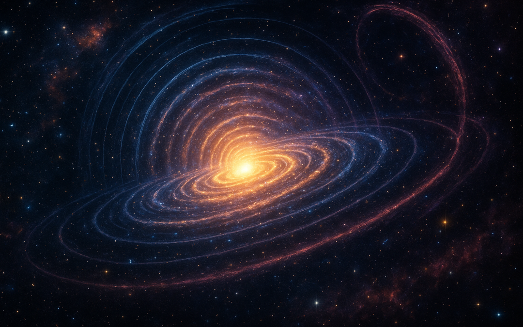
Hero — Radial Layers with Logarithmic Arms (turn-based)

Cosmic radial layers with logarithmic spiral arms Concentric radial layers and two opposite turn-based logarithmic spiral arms r=a·e^{βu}.
Figure 0 — Radial layers with two opposite logarithmic spiral arms r=a\,e^{\beta u}.

Radial Mapping of Stellar and Galactic Systems

Galaxies and clusters frequently exhibit radial or pseudo-radial structure. GRG models such systems as cumulative radial layers:

$$ \rho(r)=\sum_{k=1}^{N} f_k(r) $$

This representation captures luminosity gradients and supports multi-scale “zoom” without discontinuities.

Dark Matter Distribution

Halo profiles are commonly modeled by radial functions such as the Navarro–Frenk–White (NFW) profile:

$$ \rho_{\mathrm{NFW}}(r)\;=\; \frac{\rho_0}{\big(\tfrac{r}{r_s}\big)\,\big(1+\tfrac{r}{r_s}\big)^2} $$

In GRG, synthetic halos arise from discrete radial accumulation, enabling efficient comparisons with survey data.

Gravitational Lensing Simulations

Deflection stems from radial potentials. Under GRG, a quick discretized approximation is:

$$ \vec{\alpha}(r)\;\propto\;\frac{M(r)}{r^2}\,\vec{r} $$

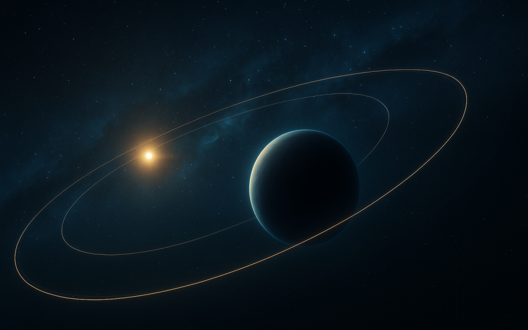
where M(r) is the generative radial mass. The map below shows curved light-ray paths and equipotential-like curves around a central mass.

Gravitational lensing map (radial potential) A central mass with families of equipotential-like curves and bent light paths.
Figure 2 — Radial potential and light deflection.

Spherical Surveys and Data Navigation

Large surveys (e.g., GAIA) live in spherical coordinates. GRG promotes seamless inside-out navigation using radial and angular indexing:

$$ \begin{aligned} \text{radial index:}\quad& z_k = k\,\Delta z,\; k=0,\dots,N_z \\ \text{angular index:}\quad& u_j = j\,\Delta u,\; \Delta u=\tfrac{1}{N_u} \\ \text{radial bound:}\quad& \rho_k=\sqrt{R^2-z_k^2} \end{aligned} $$

This allows continuous navigation across scales and directions without discontinuities.

Radial and angular indexing for spherical surveys Concentric rings and angular sectors; sample stars mark indexed bins.
Figure 3 — Rings + angular sectors for within-r queries and multi-resolution bins.

Computational Benefits

  • Multi-scale coherence: continuous zoom from core to periphery
  • Simplified algorithms in radial/turn coordinates
  • Natural fit for circular or spherical symmetries
  • Efficient indexing and clustering (e.g., “find all stars within r = 5 pc”)
  • Digital-native arithmetic: sums and square roots, π-free

Conclusion

Applying GRG to astronomy yields natural models of cosmic structure, high-fidelity simulations, and streamlined analysis pipelines. It couples geometric intuition with computational efficiency and offers a practical language for radial phenomena.
GRG for ellipses

GRG for ellipses

GRG for Ellipses — Constructive Area, Perimeter, and Equal-Area Sectors

The “Variable Radius” in GRG

The effective radius depends on the chosen direction.

  • From the center (angle \(\phi\) from the major axis):

    $$ r_c(\phi)=\frac{ab}{\sqrt{(b\cos\phi)^2+(a\sin\phi)^2}}. $$
  • From the focus (true anomaly \(\theta\)):

    $$ r_f(\theta)=\frac{p}{1+e\cos\theta},\qquad e=\sqrt{1-\frac{b^2}{a^2}},\qquad p=\frac{b^2}{a}. $$
  • Without trigonometry (slope \(m=\tan\phi\)):

    $$ r_c(m)=\frac{ab\,\sqrt{1+m^2}}{\sqrt{\,b^2+a^2m^2\,}}. $$

Ellipse Area in GRG

A1) Cartesian strips in the first quadrant

Split the semi-axis \(a\) into \(N\) parts: \(x_i=i\,a/N\) with \(\Delta x=a/N\). Heights \(y_i=b\sqrt{1-x_i^2/a^2}\).

$$ A_{1/4}^{(N)}=\sum_{i=1}^{N} y_i\,\Delta x,\qquad A^{(N)}=4\,A_{1/4}^{(N)}. $$
A1 — Cartesian strips in the first quadrant x–y axes, ellipse centered at (400,250) with a=240, b=160; shaded vertical strip inside Q1. +y +x Cartesian strips in Q1; then ×4
Quarter-by-strips: sum \(y_i\,\Delta x\) in Q1 and multiply by 4 for the ellipse area.

A2) Radial wedges from the center (by quarters)

With \(\Delta\phi=90^\circ/N\) and \(\phi_i=i\,\Delta\phi\):

$$ A_{1/4}^{(N)}=\sum_{i=0}^{N-1}\tfrac12\,r_c(\phi_i)\,r_c(\phi_{i+1})\,\sin\Delta\phi, \qquad A^{(N)}=4\,A_{1/4}^{(N)}. $$
A2 — Center-based wedges (quarter symmetry) Rays from center to ellipse boundary; the wedge between two rays approximates an area piece. C +x +y Center-based wedges (quarter symmetry)
Sum center-based wedges over a quarter (then ×4). Summing the chords between successive boundary points gives the corresponding perimeter.

A3) Radial wedges from the focus (natural for orbits)

With \(\Delta\theta=360^\circ/M\) and \(\theta_i=i\,\Delta\theta\):

$$ A^{(M)}=\sum_{i=0}^{M-1}\tfrac12\,r_f(\theta_i)\,r_f(\theta_{i+1})\,\sin\Delta\theta. $$
A3 — Focus-based sectors (equal areas → equal times) Sectors with apex at a focus; each filled sector has the same area increment ΔA (Kepler-2). F F′ periapsis → Equal-area sectors from the focus (constant ΔA; angle widths vary)
Equal-area stepping from the focus: constant \(\Delta A\) gives uniform time steps (Kepler’s 2nd law). Near periapsis the angular gaps shrink; away they widen.

Perimeter (sum of chords)

P1) Chords from the center (by quarters)

With \(\Delta\phi=90^\circ/N\):

$$ P_{1/4}^{(N)}=\sum_{i=0}^{N-1}\sqrt{\,r_c(\phi_i)^2+r_c(\phi_{i+1})^2-2\,r_c(\phi_i)\,r_c(\phi_{i+1})\cos\Delta\phi\,}, \qquad P^{(N)}=4\,P_{1/4}^{(N)}. $$

P2) Chords from the focus (full ellipse)

$$ P^{(M)}=\sum_{i=0}^{M-1}\sqrt{\,r_f(\theta_i)^2+r_f(\theta_{i+1})^2-2\,r_f(\theta_i)\,r_f(\theta_{i+1})\cos\Delta\theta\,}. $$

GRG Error Estimate (after-the-fact)

With step doubling the error typically decays ~quadratically. Method-agnostic (π-free):

  • Compute \(S_N\) and \(S_{2N}\) with the same operator (A1–A3, P1–P2).

  • Accelerated approximation:

    $$ S_\star \approx S_{2N}+\frac{S_{2N}-S_N}{3}. $$
  • Error estimate:

    $$ \varepsilon \approx \frac{|S_{2N}-S_N|}{3}. $$

Practical Pipeline (geometry → orbits)

  • Geometry: use A1 or A2 for area and P1 for perimeter with quarter symmetry.

  • Orbits: use A3. For uniform time steps, enforce constant-area sectors:

    $$ \tfrac12\,r_f(\theta_k)\,r_f(\theta_{k+1})\,\sin(\theta_{k+1}-\theta_k)=\Delta A. $$
  • The arc length per step is the P2 chord between successive points.