
Radius, Rotation, Arc

Radius, Rotation, Arc

Generative Radial Geometry: Radius, Rotation, and Arc Length

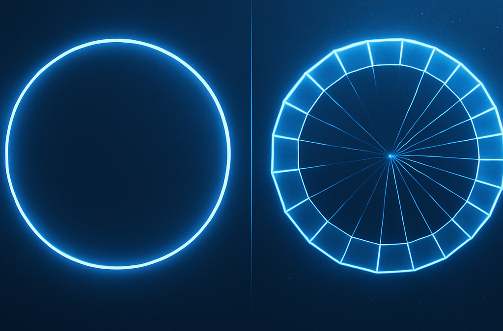
Generative Radial Geometry (GRG) provides a discrete, π-free, constructive method to generate circles, spheres, and related shapes. Instead of assuming π and continuous formulas, GRG builds geometry from radial divisions, summing chords and trapezoids. This creates a radically different perspective compared to the classical approach. Angles are expressed as fractions of the turn ($u\in[0,1)$).

Why GRG Matters

Classical geometry relies on π and continuous trigonometric functions. GRG, in contrast, is digital-native: it works with finite steps, exact points on the circumference, and simple arithmetic operations. This makes it both conceptually new and computationally efficient.

Core Comparison

The table below highlights the key differences between the two approaches.

Aspect Classical Approach Generative Radial Geometry (GRG)
Definition of angle Radians \((s=r\theta)\) with \(\pi\). Angle = discrete fraction \(k/N\) of the turn \((u\in[0,1))\), generated internally.
Mathematical tools Trigonometry, sine/cosine, continuous integrals. Finite sums of chords and trapezoids; additions and square roots.
Points on the circle Require trig functions (numerically approximated). Exact by construction on generated radial sets \((x^2+y^2=R^2)\).
Lengths and areas Closed forms: \(s=r\theta\), \(A=\pi R^2\). Generated sums: \(L=\sum \ell_i\), \(A=\sum A_i\); \(\pi\) emerges as a limit.
Local error None in theory, but depends on \(\pi\)/trig numeric precision. Error only from finite sums; boundary points remain exact.
Extension to 3D New formulas needed (e.g., \(V=\tfrac{4}{3}\pi R^3\)). One constructive scheme extends to surfaces and volumes.
Computational efficiency Expensive trig; slower on low-level hardware. Roots + sums; friendly to SIMD/GPU and embedded devices.
Concept of \(\pi\) \(\pi\) assumed a priori. \(\pi\) appears from the discrete generative process.
Conceptual view Geometry as a static entity to be measured. Geometry as an internal, generative process.

Three GRG Modes

On this page we use three operational modes. Two are Cartesian and compute area on a quarter (by symmetry). One is radial and computes circumference on the full turn.

Mode Target Partition Element Estimate Formula (sketch) Notes
Δx Trapezoidal (Cartesian) Area Quarter, \(x_i=i\,\Delta x\), \(\Delta x=R/N\) Trapezoids between heights \(h_i=\sqrt{\,R^2-x_i^2\,}\) Lower (under-tiling) \(A_Q \approx (\Delta x/2)\sum(h_i+h_{i+1})\); total area \(=4\,A_Q\) Monotone ↑ with \(N\)
Projection Corridor (Cartesian) Area Quarter, same \(\Delta x\) Riemann-like bars at right / midpoint Lower/Upper (squeezing) \(A_Q^{\downarrow}=\Delta x\sum h_i\), \(A_Q^{\uparrow}=\Delta x\sum h_{i+\tfrac12}\); total \(=4\times\) Certified bounds
Chord-Sum at \(\Delta u\) (Radial) Circumference Full turn, \(\Delta u=1/N\) Chords between consecutive radial points Lower (inscribed polygon) \(L \approx N\,R\,\sqrt{\,2-2\,c(1/N)\,}\) No quarter; defined on the whole circle
Note on “quarters”. The quarter is used only for the Cartesian area modes (by symmetry). For circumference we operate on the full turn (radial partition), so “quarters” are not meaningful there.

Further Evaluations & Options

  • Certified area bounds. The corridor (right vs midpoint) yields lower/upper bounds that squeeze the exact area as \(N\) grows.
  • Stronger circumference bracketing. Pair the inscribed chord-sum (lower) with a circumscribed tangent-sum (upper) to bound the true length.
  • Adaptive refinement. Increase \(N\) only where variation is largest (near endpoints for Cartesian area; uniform \(\Delta u\) usually suffices for chords).
  • Hybrid pipelines. Use circumference from chords to cross-check the discrete derivative of area w.r.t. \(R\).
  • 3D extension. The same logic generalizes to spherical belts (length) and frusta/patch sums (area/volume) with discrete radial partitions.
  • Hardware efficiency. All modes need only sums and square roots → ideal for embedded, SIMD, and GPU kernels.

Conclusions

Classical geometry excels in closed-form elegance. GRG complements it with a digital-native, constructive view: exact boundary points, sums that converge without assuming π, and a single scheme that scales from 2D to 3D. Here we use three GRG modes—two Cartesian for area on a quarter, one radial for circumference on the full turn—unlocking certified bounds, adaptive strategies, and hardware-friendly implementations.

Inside-Out GRG

Inside-Out GRG

GRG — Looking from the Inside: a discrete, π-free language for shapes

Generative Radial Geometry (GRG) — Looking from the Inside

GRG conventions. Angles are measured in turns \(u\in[0,1)\). Radial computations (perimeter and radial area) run on the full turn; the Cartesian area uses the quarter (and then ×4). Trigonometric forms are optional cross-checks, not inputs to the pipeline.

Work-in-progress. GRG is a discrete, π-free way to measure and compare shapes by radial generation. The turning point was this: I looked at the circle from its inside—a point that sends rays outward and measures what they meet. That inside→out switch is small to say and large to practice. The door is open; we will walk through it.

Why GRG matters

  • Discrete by nature: everything runs in finite steps (N)—heights, chords, bands.
  • π-free computation: the pipeline never needs π to run; π appears only when we compare to classical values.
  • Immediate comparability: two shapes at the same resolution are directly comparable with the same grammar.
  • Multi-scale: increase N; the very same procedure refines itself (coarse → fine).
  • GPU-friendly: short loops and sums, ideal for digital geometry, CAD/graphics, and simulation.

Looking from the inside

Not from a grid of squares, not from external coordinates—from a center that emits rays. A shape becomes a radial profile (a finite vector of values) rather than a formula to solve. From there, measurement and comparison happen discretely and immediately.

The joined method (circle)

Perimeter (radial, full turn): split the full turn \(u\in[0,1)\) into \(4N\) equal steps \(\Delta u=1/(4N)\). Join successive GRG border nodes by chords; the quarter view in the figure is for clarity.

Area (Cartesian, quarter): split one radius into \(N\) parts; at each split, drop the perpendicular to the circle (the “height”). Adjacent heights form a trapezoid; summing them tiles the quarter of a disk (the last one degenerates to a triangle). Multiply by 4 for the full disk.

Figure — joined method (circle)

Blue = angular sectors (perimeter, shown on the quarter). Red = single-radius trapezoids (area on the quarter). Dashed red rays start from the height intersections and generally do not coincide with the blue rays.

Figure 1. Quarter circle built from angular sectors (blue) and single-radius trapezoids (red); dashed rays start at height intersections.

Discrete comparability (the practical power)

At the same resolution N, any two shapes share the same grammar (heights, chords). This makes them comparable immediately—π-free inside the computation. We use simple, discrete indices relative to a baseline circle at the same N:

  • Area Index \(a_N\)
  • Perimeter Index \(c_N\)
  • Isoperimetric-like ratio \(q_N=a_N/c_N^2\) (the circle maps to 1 at the same N)
Minimal math — turns-first (π-free, node-based)

Quarter nodes (turns):

\[ \Delta u \;=\; \frac{1}{4N} \] \[ u_k \;=\; k\,\Delta u \quad (k=0,\dots,N) \]

Quarter inscribed perimeter (node distances):

\[ C_{\mathrm{in}}^{(Q)}(N) \;=\; \sum_{k=0}^{N-1} \bigl\|\,P_{k+1}-P_k\,\bigr\| \]

Full inscribed perimeter:

\[ C_{\mathrm{in}}(N) \;=\; 4\,C_{\mathrm{in}}^{(Q)}(N) \]

Radial area (full turn, shoelace on 4N nodes):

\[ A_{\mathrm{in}}(N) \;=\; \frac{1}{2} \sum_{j=0}^{4N-1} \bigl(x_j\,y_{j+1}-x_{j+1}\,y_j\bigr) \]

Cartesian area (quarter, Δx) → ×4:

\[ \Delta x \;=\; \frac{R}{N} \] \[ x_i \;=\; i\,\Delta x \] \[ y_i \;=\; \sqrt{\,R^2 - x_i^{\,2}\,} \] \[ A_{\mathrm{trap}}^{(Q)}(N) \;=\; \sum_{i=1}^{N} \frac{y_{i-1}+y_i}{2}\;\Delta x \] \[ A_{\mathrm{trap}}(N) \;=\; 4\,A_{\mathrm{trap}}^{(Q)}(N) \]

Discrete indices (baseline = circle at the same N):

\[ a_N \;=\; \frac{A_{\text{shape}}(N)}{A_{\text{circle}}(N)} \] \[ c_N \;=\; \frac{C_{\text{shape}}(N)}{C_{\text{circle}}(N)} \] \[ q_N \;=\; \frac{a_N}{c_N^{\,2}} \]
Classical cross-check (optional)

Inscribed perimeter (quarter step in turns):

\[ \Delta u \;=\; \frac{1}{4N} \] \[ s_N \;=\; 2R\,\sin\!\bigl(\pi\,\Delta u\bigr) \] \[ C_{\mathrm{in}}(N) \;=\; 4\,N\,s_N \;=\; 8\,N\,R\,\sin\!\Bigl(\frac{\pi}{4N}\Bigr) \]

Circumscribed perimeter (outer bound):

\[ C_{\mathrm{out}}(N) \;=\; 8\,N\,R\,\tan\!\Bigl(\frac{\pi}{4N}\Bigr) \]

Radial area via triangles (full turn):

\[ A_{\mathrm{tri}}(N) \;=\; 2\,N\,R^{2}\, \sin\!\Bigl(\frac{\pi}{2N}\Bigr) \]

Cartesian area (quarter, Δx) — same as above, then ×4.

Figure — 3D comparator (hemisphere bands)

Clean comparator for surfaces: baseline hemisphere on the left, target surface on the right. Blue = GRG parallels on each latitude; red = bands (average of neighboring circumferences). Below, π-free indices (schematic bars).

Figure 2. Hemisphere bands comparator: left = baseline, right = target. Blue parallels indicate perimeter along latitude; red band shows area via average neighboring circumferences times slant. Bars below sketch π-free indices.

From the circle to the sphere (concept)

We stack latitude bands along the vertical axis and apply the same grammar on each parallel (GRG circumference on the band’s ends, averaged across the slant). Errors shrink fast with balanced vertical and angular splits. The comparator above is designed to show differences band-by-band without clutter.

Applications

  • Graphics/CAD: π-free arc lengths and areas that run fast and parallel.
  • Sampling/tiling on spheres: controllable bands, equal-area approximations.
  • Gear-like and elliptical profiles via directional radial generation.
  • Education: a concrete bridge from discrete geometry to classical values.

Status & invitation

GRG is young and grows with this site. The aim is simple: a practical, comparable, discrete language for shapes and surfaces. If the idea helps, let’s refine proofs, diagrams, and applications together.