
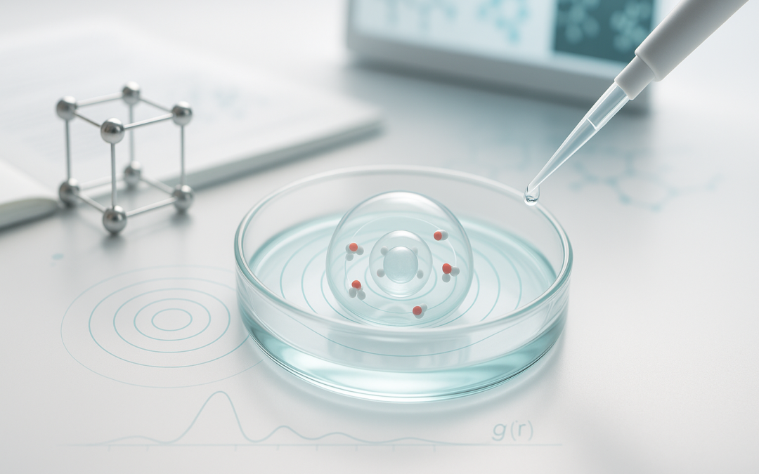
Chemistry
Generative Radial Geometry for Chemistry: From Conformers to MOFs and Solvent Shells
Generative Radial Geometry (GRG) offers a center-out way to construct and search chemical structures. By organizing atoms, coordination sites, pores, or solvent molecules in radial shells with controlled distances and angles, GRG cuts down the combinatorial explosion and makes 3D models that are physically plausible and immediately ready for simulation.
Where GRG helps in chemistry
- Molecule modeling & design: targeted conformer generation around rings and chiral centers; pre-screening of virtual libraries to propose sterically sensible radial scaffolds.
- Crystallography & solids: crystal packing via radial neighborhoods of a repeat unit; localized models of defects and vacancies.
- Molecular dynamics: fast computation of radial distribution functions (RDF) and balanced initialization of solvents/ions around a solute.
- Porous materials (MOF/COF): radial placement of metal nodes around linkers; geometric control of free radii to tune pore accessibility.
- Supramolecular self-assembly: prediction of micelles/liposomes and core–shell architectures by concentric, composition-aware layers.
- Drug design & docking: radial abstractions of binding pockets and “radial grids” of electrostatic potential to guide polar/apolar moieties.
Δx Trapezoidal (Cartesian)
Target: fast area/volume roll-ups • Estimate: lower • Domain: quarter (×4)
- RDF histograms (shell counts), coordination numbers (baseline).
- Solvent occupancy per shell; pore cross-section scans.
Projection Corridor
Target: certified bounds on integrals • Estimate: lower & upper • Domain: quarter (×4)
- Bounds for \(N(R)=4\pi\rho\!\int_0^R\!g(r)\,r^2dr\) and shell occupancies.
- Stop when gap ≤ tolerance; use to compare force fields robustly.
Chord-Sum at Δu (Radial)
Target: ring/loop sampling & perimeter • Estimate: lower (add tangent-sum ↑) • Domain: full turn
- Uniform directions \(u\in[0,1)\) for conformers/solvent placement.
- Pore apertures & ring tiling in MOFs/COFs; angular RDF slices.
Picker by task. Need speed → Trapezoid; need guarantees/threshold radii → Corridor; need angular uniformity/phase on rings → Chord-Sum (± tangent-sum); volumetrics → shell/belt extensions.
Core GRG idea for chemical systems
Place partners within radial bounds and enforce angular/steric constraints; then score candidates and iterate. Typical constraints:
$$ r_{\min} \;\le\; r \;\le\; r_{\max}, \qquad \angle(\text{A–C–B}) \;\ge\; \alpha_{\min}. $$For distributions, the classic RDF (pair correlation) reads:
$$ g(r) \;=\; \frac{1}{4\pi r^{2}\,\rho\,N}\, \sum_{i\ne j}\, \delta\!\bigl(r-\lVert \mathbf{r}_i-\mathbf{r}_j \rVert \bigr). $$GRG modes: Use Trapezoid to accumulate RDF shell counts quickly; switch to Corridor for certified bounds on coordination \(N(R)=4\pi\rho\!\int_0^R\!g(r)\,r^2dr\); use Chord-Sum at \(\Delta u=1/N\) to ensure uniform angular sampling when RDF is evaluated over directional sectors.
Worked examples
1) Conformer generation around a chiral center
Goal: explore the spatial arrangements around a chiral carbon and select the most stable isomer.
- Define the chiral center C and the four substituents (A, B, C, D).
- Choose distance bounds for C–X: e.g., 1.45–1.55 Å.
- Partition the interval into k concentric shells (e.g., 5).
- On each shell, sample directions with turns \(u\in[0,1)\) at \(\Delta u=1/N\), enforcing tetrahedral angles ≈\(109.5^\circ\) and min separations.
- Score with a light force field (e.g., UFF) and retain the lowest-energy 10 conformers.
GRG modes: Chord-Sum (full turn, turns \(u\)) for uniform angular sampling and ring-wise sterics; Trapezoid to tally shell feasibility quickly; Corridor to certify bounds on steric/energy scores over shells before QM refinement.
2) Crystal packing of a simple MOF
Goal: arrange metal nodes and organic linkers in a cubic unit cell using radial symmetry.
- Place a metal node M (e.g., Zn2+) at the cell center; four linkers L at the corners of a radial tetrahedron.
- Set coordination bounds (e.g., M–O = 1.9–2.2 Å).
- For each L site, sample positions on a spherical shell about M, keeping \(\angle\text{L–M–L}\approx 109.5^\circ\).
- Tile the cell periodically with vectors \((a,0,0)\), \((0,a,0)\), \((0,0,a)\).
- Run a short geometry minimization (e.g., Powell) to relieve strain.
GRG modes: Chord-Sum for ring apertures and angular registry of linkers (periodic tiling over full turn); Trapezoid for cross-sectional pore area scans (quarter ×4); Corridor to bound pore-limiting/free-sphere radii derived from those scans.
3) Solvent bubble for MD around a solute
Goal: generate a balanced water sphere around a charged solute without overcrowding.
- Locate the solute center of mass and choose \(R_1\) (solute + first shell) and \(R_2\) (outer boundary).
- Split \([R_1,R_2]\) into \(N\) shells (typically 3–5).
- For each shell, place water molecules by sampling directions uniformly with turns \(u\) and \(\Delta u=1/N\); set distances \(r\) within that shell and enforce \(d_{\min}(\mathrm{O}, \text{solute}) \ge 2.5\ \text{Å}\).
- Assign water orientations (H–O–H) with small random perturbations.
- Export to PDB and run a short heating/minimization to relax the sphere.
GRG modes: Chord-Sum for uniform angular placement/orientations; Trapezoid for quick shell occupancy and radial density; Corridor to bracket hydration numbers \(N(R)\) and to stop when bounds meet your tolerance.
4) Docking on radial electrostatic grids (quick setup)
Goal: approximate binding pocket neighborhoods with radial shells and guide pose sampling.
- Center a pocket reference and define shells \([r_k,r_{k+1}]\) plus ring samples at turns \(u_j=j/N\).
- Precompute coarse electrostatic potential on these cells; score ligand fragments by shell and ring.
- Promote top cells to fine sampling; enforce sterics and ring-wise clashes; export poses to your docking engine.
GRG modes: Chord-Sum for ring coverage of orientations; Trapezoid to roll up cell scores radially; Corridor to keep upper/lower envelopes on pocket accessibility/energy as you refine.
From generation to computation
- Search space reduction: symmetries and radial bounds focus the exploration on chemically sensible regions.
- 3D realism with control: enforce minimum/maximum inter-center distances and angles while sampling.
- Drop-in to pipelines: GRG output meshes with QM, MD, and docking workflows (e.g., UFF pre-screen → PDB export → MD heating → production run).
GRG modes (pipeline): Use Trapezoid during fast scans; switch to Corridor to certify thresholds (coordination/hydration/pore radii); validate angular uniformity/perimeters with Chord-Sum (± tangent-sum) before committing to costly runs.
Conclusion
Across molecular design, crystal engineering, porous frameworks, self-assembly, and simulation setup, GRG brings a clear center-out logic: define radial bounds, discretize into shells, generate angles under constraints, and score. Choosing among Δx Trapezoidal, Projection Corridor, and Chord-Sum at Δu—or combining them—yields fast baselines, certified bounds, and robust angular control for meaningful chemistry.
RDF & Coordination via GRG Corridor — bounds on N(R) and Rn
Definitions. With bulk number density \(\rho\) and radial distribution \(g(r)\), the coordination number inside radius \(R\) is
$$ N(R)=4\pi\rho\int_0^{R} g(r)\,r^2\,dr. $$Discrete GRG shells. Choose radii \(0=r_0
Corridor bounds (cumulative up to \(R\)).
$$ N^{\downarrow}(R)=\rho\!\!\sum_{k:\,r_{k+1}\le R}\! V_k\,g_k^{\min},\qquad N^{\uparrow}(R)=\rho\!\!\sum_{k:\,r_{k+1}\le R}\! V_k\,g_k^{\max}, $$Bracketing a coordination radius. For a target coordination \(n\) (e.g., “first shell”):
- \(R_{n}^{-}=\min\{R:\,N^{\uparrow}(R)\ge n\}\) is a lower bound of the true \(R_n\).
- \(R_{n}^{+}=\min\{R:\,N^{\downarrow}(R)\ge n\}\) is an upper bound of the true \(R_n\).
- Refine by halving shell width \(\Delta r\) near the bracket or by bisecting within the shell until \(R_{n}^{+}-R_{n}^{-}\le\) tolerance.
Method picker. Isotropic liquids: use shells only (fast). Structured/anisotropic systems or near interfaces: split shells into polar cells; sample azimuth with Chord-Sum (\(\Delta u=1/N\)) to keep directional coverage, then apply the corridor per cell. Use Trapezoid for quick scans of \(N(R)\); switch to Corridor when you need guarantees.
Practical notes. Use \(\Delta r\) small enough to resolve the first peak of \(g(r)\) (typ. 0.02–0.05 nm); respect PBC and the minimum-image convention (limit \(R\le L/2\) in a cubic box). For noisy \(g(r)\), smooth lightly after computing corridor bounds, not before.