A Symmetric GRG Kernel for Area

Jun 17, 2026

A Symmetric GRG Kernel for Area

The binary radial formulation combines complementary internal and external sector triangles. The area kernel uses one internal contribution and two external contributions, unlike the circumference kernel’s two-to-one chord–tangent balance.

Geometric Elements

Resolve one Turn into N equal symmetric sectors. Let a be the internal triangle’s height, h half its chord, and e half the external tangent side. Define q = h/a.

$$
N=2^b,\quad b\ge2,\quad R>0,\qquad a^2+h^2=R^2,\quad e=R\frac ha.
$$

$$
I_b=ah=R^2\frac{q_b}{1+q_b^2},\qquad E_b=Re=R^2q_b.
$$

Two Area Kernels

$$
A_m=\frac N2(I_b+E_b),\qquad A_w=\frac N3(I_b+2E_b).
$$

Accuracy for the Defined Triangles

The current formulation gives an analytical verification using a local integral as an exact sector reference, not as a kernel input.

$$
F(q)=\int_0^q\frac{dt}{1+t^2},\qquad A_T(R)=NR^2F(q_b).
$$

$$
\begin{aligned}A_m-A_T&=NR^2\left(-\frac{q_b^3}{6}+\frac{3q_b^5}{10}+O(q_b^7)\right),\\A_w-A_T&=NR^2\left(\frac{2q_b^5}{15}+O(q_b^7)\right).\end{aligned}
$$

Regular geometric bisection yields a scale bound. Together with the expansion, it proves second-order total error for the arithmetic kernel and fourth-order total error for the weighted kernel in exact arithmetic.

$$
0\lt q_b\le\frac4N,\qquad A_m-A_T=O(N^{-2}),\qquad A_w-A_T=O(N^{-4}).
$$

The same analysis proves the following bracket for these sectors:

$$
A_{\mathrm{in}}\le A_m\le A_T\le A_w\le A_{\mathrm{out}}.
$$

Sampling and Scope

$$
\Delta u=\frac1{4N}.
$$

The earlier version introduced this quarter-step sampling parameter inside each module. The proof here concerns the complete sector triangles defined above. A different sample-based area construction requires its own explicit definition and proof.

Internal–external weights are reversed between the circumference and area kernels. This diagram is schematic; the triangle definitions determine the calculation.

Research Status

The cancellation is established for the regular triangular elements above. This does not establish original authorship of the weighting, numerical stability of an implementation, or a computational advantage. Those questions require separate literature and implementation comparisons.

Earlier revisions of this page described fourth-order behaviour as a candidate. The current analytical clarification identifies the geometric assumptions under which that behaviour follows.

Radius, Rotation, Arc

Sep 7, 2025

Generative Radial Geometry: Radius, Rotation, and Arc Length

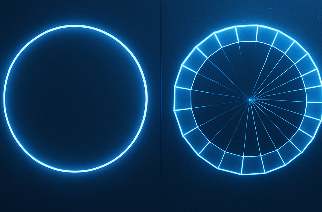
Generative Radial Geometry (GRG) provides a discrete, π-free, constructive method to generate circles, spheres, and related shapes. Instead of assuming π and continuous formulas, GRG builds geometry from radial divisions, summing chords and trapezoids. This creates a radically different perspective compared to the classical approach. Angles are expressed as fractions of the turn ($u\in[0,1)$).

Why GRG Matters

Classical geometry relies on π and continuous trigonometric functions. GRG, in contrast, is digital-native: it works with finite steps, exact points on the circumference, and simple arithmetic operations. This makes it both conceptually new and computationally efficient.

Core Comparison

The table below highlights the key differences between the two approaches.

Aspect	Classical Approach	Generative Radial Geometry (GRG)
Definition of angle	Radians $(s=r\theta)$ with $\pi$.	Angle = discrete fraction $k/N$ of the turn $(u\in[0,1))$, generated internally.
Mathematical tools	Trigonometry, sine/cosine, continuous integrals.	Finite sums of chords and trapezoids; additions and square roots.
Points on the circle	Require trig functions (numerically approximated).	Exact by construction on generated radial sets $(x^2+y^2=R^2)$.
Lengths and areas	Closed forms: $s=r\theta$, $A=\pi R^2$.	Generated sums: $L=\sum \ell_i$, $A=\sum A_i$; $\pi$ emerges as a limit.
Local error	None in theory, but depends on $\pi$/trig numeric precision.	Error only from finite sums; boundary points remain exact.
Extension to 3D	New formulas needed (e.g., $V=\tfrac{4}{3}\pi R^3$).	One constructive scheme extends to surfaces and volumes.
Computational efficiency	Expensive trig; slower on low-level hardware.	Roots + sums; friendly to SIMD/GPU and embedded devices.
Concept of $\pi$	$\pi$ assumed a priori.	$\pi$ appears from the discrete generative process.
Conceptual view	Geometry as a static entity to be measured.	Geometry as an internal, generative process.

Three GRG Modes

On this page we use three operational modes. Two are Cartesian and compute area on a quarter (by symmetry). One is radial and computes circumference on the full turn.

Mode	Target	Partition	Element	Estimate	Formula (sketch)	Notes
Δx Trapezoidal (Cartesian)	Area	Quarter, $x_i=i\,\Delta x$, $\Delta x=R/N$	Trapezoids between heights $h_i=\sqrt{\,R^2-x_i^2\,}$	Lower (under-tiling)	$A_Q \approx (\Delta x/2)\sum(h_i+h_{i+1})$; total area $=4\,A_Q$	Monotone ↑ with $N$
Projection Corridor (Cartesian)	Area	Quarter, same $\Delta x$	Riemann-like bars at right / midpoint	Lower/Upper (squeezing)	$A_Q^{\downarrow}=\Delta x\sum h_i$, $A_Q^{\uparrow}=\Delta x\sum h_{i+\tfrac12}$; total $=4\times$	Certified bounds
Chord-Sum at $\Delta u$ (Radial)	Circumference	Full turn, $\Delta u=1/N$	Chords between consecutive radial points	Lower (inscribed polygon)	$L \approx N\,R\,\sqrt{\,2-2\,c(1/N)\,}$	No quarter; defined on the whole circle

Note on “quarters”. The quarter is used only for the Cartesian area modes (by symmetry). For circumference we operate on the full turn (radial partition), so “quarters” are not meaningful there.

Further Evaluations & Options

Certified area bounds. The corridor (right vs midpoint) yields lower/upper bounds that squeeze the exact area as $N$ grows.
Stronger circumference bracketing. Pair the inscribed chord-sum (lower) with a circumscribed tangent-sum (upper) to bound the true length.
Adaptive refinement. Increase $N$ only where variation is largest (near endpoints for Cartesian area; uniform $\Delta u$ usually suffices for chords).
Hybrid pipelines. Use circumference from chords to cross-check the discrete derivative of area w.r.t. $R$.
3D extension. The same logic generalizes to spherical belts (length) and frusta/patch sums (area/volume) with discrete radial partitions.
Hardware efficiency. All modes need only sums and square roots → ideal for embedded, SIMD, and GPU kernels.

Conclusions

Classical geometry excels in closed-form elegance. GRG complements it with a digital-native, constructive view: exact boundary points, sums that converge without assuming π, and a single scheme that scales from 2D to 3D. Here we use three GRG modes—two Cartesian for area on a quarter, one radial for circumference on the full turn—unlocking certified bounds, adaptive strategies, and hardware-friendly implementations.

GRG Trapezoidal

Sep 6, 2025

Earlier Formulation

This page preserves a historical GRG method. Its notation and formulas belong to that version. The current binary radial formulation and verification are available here. Historical computational claims require separate validation.

Δx Trapezoidal

This GRG block computes the circle’s area from the inside using uniform $\Delta x=r/N$ on the quarter. On the graph $y(x)=\sqrt{r^{2}-x^{2}}$, adjacent samples form trapezoids strictly under the arc; multiply by $4$ for the full circle. No angles are required and no external constants appear in the primary formulas.

Setup

$$ \Delta x \;=\; \frac{r}{N}, \qquad x_k \;=\; k\,\Delta x \quad (k=0,\dots,N), \qquad y_k \;=\; \sqrt{\,r^{2}-x_k^{2}\,}. $$

Fig. 1 — Δx trapezoids strictly inside the quarter arc (N=5).

Quarter-area sum (→ ×4 for the circle)

$$ A_{\text{quarter}}(N) \;=\; \sum_{k=0}^{N-1} \frac{\Delta x}{2}\,\bigl( y_k + y_{k+1} \bigr), \qquad A_{\text{circle}}(N) \;=\; 4\,A_{\text{quarter}}(N). $$

Fig. 2 — One Δx trapezoid; the dashed arc shows the exact curve above it.

Why use this block

Monotone under-approximation (trapezoids are strictly inside the quarter arc).
Smooth convergence $\sim O(N^{-2})$ and numerically stable (simple sums and square roots).
No angle handling; easy to implement with fixed-point or vectorized code.

How to use

Choose $N$ (e.g., $200$–$1000$) to balance speed and accuracy.
Step-doubling check: compare results at $N$ and $2N$ to gauge the remaining gap.
Optional diagnostic: plot the trapezoids on the quarter to see the under-tiling.

Notes

The last strip degenerates to a triangle since $y_N=0$ at $x_N=r$.
Perimeter pairs naturally with equal-angle chords; see the Core Turns block for the chord formula.

See also: Core Turns · Original Projection · Applications / Circle

Δx Trapezoidal

Area from the inside: sample the quarter with uniform $\Delta x = r/N$, use trapezoids under the arc on $y(x)=\sqrt{r^{2}-x^{2}}$, then multiply by $4$ for the full circle. No angles required.

Formula box — Quarter setup

$$ \Delta x \;=\; \frac{r}{N}, \qquad x_k \;=\; k\,\Delta x \ \ (k=0,\dots,N), \qquad y_k \;=\; \sqrt{\,r^{2}-x_k^{2}\,}. $$

Formula box — Quarter area (→ ×4)

$$ A_{\text{quarter}}(N) \;=\; \sum_{k=0}^{N-1} \frac{\Delta x}{2}\,\bigl[\,y_k + y_{k+1}\,\bigr] $$

$$ A_{\text{circle}}(N) \;=\; 4\,A_{\text{quarter}}(N) $$

Properties

Monotone under-approximation: each trapezoid lies strictly inside the quarter arc.
Convergence $\sim O(N^{-2})$. Numerically stable: sums and square roots only.
The last strip degenerates to a triangle because $y_N=0$ at $x_N=r$.

How to use

Choose $N$ (e.g., $200$–$1000$) based on speed/accuracy needs.
Step-doubling check: compare results at $N$ and $2N$ to estimate the remaining gap.
Optional: plot the trapezoids on the quarter to visualize the under-tiling.

GRG Original Projection

Sep 4, 2025

Earlier Formulation

This page preserves a historical GRG method. Its notation and formulas belong to that version. The current binary radial formulation and verification are available here. Historical computational claims require separate validation.

Original Projection — historical method This page presents the original GRG idea: the circle is generated from the inside. The circle area is computed on a quadrant by projecting heights onto the x-axis and using midpoint rectangles (discrete upper); a matching right-endpoint rule gives a discrete lower, forming an under/over corridor that shrinks as $N$ increases (the midpoint rule is second-order). The perimeter is obtained from the sum of equal-angle chords on the quadrant (then $\times 4$). This method remains alongside other GRG blocks and is kept intact for comparison and continued study. See also Core Turns and Δx Trapezoidal.

Original Projection (Quarter → ×4)

Work on the quarter $x\in[0,r]$ with the profile $y(x)=\sqrt{r^{2}-x^{2}}$. Use uniform $\Delta x=r/N$. Midpoint rectangles provide a discrete upper estimate; right-endpoint rectangles provide a discrete lower. Multiply by $4$ to obtain full-circle values.

Setup

$$ \Delta x \;=\; \frac{r}{N}, \qquad x_k \;=\; k\,\Delta x \ (k=0,\dots,N), \qquad x_{k+\tfrac12} \;=\; \Bigl(k+\tfrac12\Bigr)\Delta x, \qquad y(x) \;=\; \sqrt{\,r^{2}-x^{2}\,}. $$

Quarter area: discrete corridor (upper vs lower)

Midpoint (discrete upper, second-order)

$$ A_{\text{quarter}}^{\text{mid}}(N) \;=\; \sum_{k=0}^{N-1} \Delta x \; y\!\bigl(x_{k+\tfrac12}\bigr), \qquad A_{\text{circle}}^{\text{mid}}(N) \;=\; 4\,A_{\text{quarter}}^{\text{mid}}(N). $$

Right-endpoint (discrete lower)

$$ A_{\text{quarter}}^{\text{right}}(N) \;=\; \sum_{k=0}^{N-1} \Delta x \; y\!\bigl(x_{k+1}\bigr), \qquad A_{\text{circle}}^{\text{right}}(N) \;=\; 4\,A_{\text{quarter}}^{\text{right}}(N). $$

Corridor: $A_{\text{circle}}^{\text{right}}(N) \;\le\; \text{Area(circle)} \;\le\; A_{\text{circle}}^{\text{mid}}(N)$, with gap shrinking like $O(N^{-2})$ under smoothness.

Perimeter via equal-angle chords (quadrant → ×4)

Partition the quarter by equal angular steps in turns. Let the quarter have $Q$ equal-angle chords of step $\Delta u=\tfrac{1}{4Q}$. The sum over the quarter is

$$ C_{\text{quarter}}(Q) \;=\; 2\,Q\,r\,s\!\Bigl(\tfrac{\Delta u}{2}\Bigr) \;=\; 2\,Q\,r\,s\!\Bigl(\tfrac{1}{8Q}\Bigr), \qquad C_{\text{circle}} \;\approx\; 4\,C_{\text{quarter}}(Q) \;=\; 8\,Q\,r\,s\!\Bigl(\tfrac{1}{8Q}\Bigr). $$

Equivalently, with $N=4Q$ steps on the full turn: $C_{N}=2\,N\,r\,s\!\bigl(\tfrac{1}{2N}\bigr)$ (see Core Turns).

Figure — Quarter with midpoint and right rectangles

Midpoint vs right-endpoint corridor on the quarter.

Why use this block

Explicit under/over corridor with midpoint/right rules on the quarter.
Second-order convergence for the midpoint rule ($O(N^{-2})$) with simple operations.
No angle handling; complements chord-based perimeter via equal-angle steps.

How to use

Choose $N$ (e.g., $200$–$1000$) for the quarter; multiply results by $4$ for the circle.
Step-doubling check: compare $N$ vs $2N$ to estimate the residual gap between upper and lower.
Pair with equal-angle chords on the quarter to report both area and perimeter consistently.

Original Projection

The original GRG area method: sample the quarter along the x-axis with uniform step $\Delta x=r/N$. At each sample, project the height on the circle graph $y(x)=\sqrt{r^{2}-x^{2}}$ and build discrete rectangles. Two rules create a shrinking corridor: midpoint rectangles (upper) and right-endpoint rectangles (lower). Multiply by $4$ for the full circle. No angles are required in this block.

Setup

$$ \Delta x \;=\; \frac{r}{N}, \qquad x_k \;=\; k\,\Delta x \quad (k=0,\dots,N), \qquad x_{k+\tfrac12} \;=\; \Bigl(k+\tfrac12\Bigr)\Delta x, \qquad y(x) \;=\; \sqrt{\,r^{2}-x^{2}\,}. $$

Quarter-area sums (→ ×4 for the circle)

$$ \textbf{Midpoint (upper):}\quad A_{\mathrm{mid}}^{\mathrm{q}}(N) \;=\; \sum_{k=0}^{N-1} y\!\bigl(x_{k+\tfrac12}\bigr)\,\Delta x $$

$$ \textbf{Right-end (lower):}\quad A_{\mathrm{right}}^{\mathrm{q}}(N) \;=\; \sum_{k=0}^{N-1} y\!\bigl(x_{k+1}\bigr)\,\Delta x $$

$$ \textbf{Circle totals:}\quad A_{\mathrm{mid}} \;=\; 4\,A_{\mathrm{mid}}^{\mathrm{q}}, \qquad A_{\mathrm{right}} \;=\; 4\,A_{\mathrm{right}}^{\mathrm{q}} $$

$$ \textbf{Corridor:}\quad A_{\mathrm{right}} \;\le\; A_{\mathrm{true}} \;\le\; A_{\mathrm{mid}} $$

$$ \textbf{Estimate (optional):}\quad A_{\mathrm{avg}} \;=\; \frac{A_{\mathrm{mid}}+A_{\mathrm{right}}}{2} \quad\text{(use half-gap as an error bar).} $$

Notes

$y(x)=\sqrt{r^{2}-x^{2}}$ is concave on $[0,r]$; hence midpoint gives an upper estimate and right-endpoint a lower one.
Increase $N$ to tighten the corridor; publish $A_{\mathrm{avg}}$ with its half-gap if you need an error bar.

See also: Δx Trapezoidal · Core Turns · Applications / Circle

GRG Core (Turns)

Aug 24, 2025

Earlier Formulation

This page preserves a historical GRG method. Its notation and formulas belong to that version. The current binary radial formulation and verification are available here. Historical computational claims require separate validation.

Core Turns

Angles are measured in turns (fractions of a full rotation). Primary 2D formulas use products only and avoid sexagesimal units and external constants. We write c(u), s(u) for cosine/sine with period 1 in turns (so $c(0)=1$, $s(0)=0$; $c(\tfrac{1}{4})=0$, $s(\tfrac{1}{4})=1$). Equivalently, $c(u)=\cos(2\pi u)$ and $s(u)=\sin(2\pi u)$.

Radial point

$$ P(u) \;=\; \bigl( r\cdot c(u),\; r\cdot s(u) \bigr). $$

Perimeter (equal-angle chords)

$$ C_N \;=\; 2\cdot N \cdot r \cdot s\!\Bigl(\tfrac{1}{2N}\Bigr). $$

Area (equal-angle sectors)

$$ A_N \;=\; \tfrac{1}{2}\cdot N \cdot r^{2} \cdot s\!\Bigl(\tfrac{1}{N}\Bigr). $$

How to use

Pick a precision $N$ (e.g., $256$). If you store angles as $k/2^{B}$ turns, choose $N$ that divides $2^{B}$.
Dyadic refinement: with $b\in\mathbb{N}_{\ge 0}$, set $N=2^{b}$ so the turn step is $\Delta u=2^{-b}$. Quarter sampling uses $\Delta u=\tfrac{1}{4N}=2^{-b-2}$.
Optional check (step-doubling): compare $N$ vs. $2N$ to gauge the remaining gap.

Notes

Both $C_N$ and $A_N$ increase with $N$ and converge to the circle values $2\pi r$ and $\pi r^2$; the error typically scales like $O\!\bigl((\Delta u)^2\bigr)=O(N^{-2})$.
This block pairs with the Trapezoidal and Original blocks on the Applications pages.

Figure: turns, chord, and sector

Radial point $P(u)$, equal-angle step $\Delta u=1/N$, chord $s(\tfrac{1}{2N})$, and sector $s(\tfrac{1}{N})$.

Generative Radial Geometry (GRG) — Formalisation (Turns)

GRG is a constructive, discrete framework based on full-turn angular partitions (turns). All angles are fractions of a full rotation $u\in[0,1)$. We use period-1 trigonometric functions $c(u), s(u)$ with $c(0)=1$, $s(0)=0$, $(c(\tfrac14), s(\tfrac14))=(0,1)$, and standard identities. Primary formulas contain no sexagesimal units and no external constants.

1) Setup and Notation (full turn)

Spaces. Plane $\mathbb{R}^2$ and space $\mathbb{R}^3$ with axes $x,y,z$.
Circle/Sphere. Center $O$, radius $r>0$. Circle: $x^2+y^2=r^2$. Sphere: $x^2+y^2+z^2=r^2$.
Angles. $u\in[0,1)$ turns. Turns-trigonometry: $c(u), s(u)$ with unit identities.

Fig. A — Angle $u$ (turns). Radial point $P(u)=(r\,c(u),\,r\,s(u))$.

2) Exact radial nodes (full turn)

For any $u\in[0,1)$:

Radial node

$$ P(u)\;=\;\bigl(r\,c(u),\; r\,s(u)\bigr). $$

Evenly-spaced angles: $u_k=k/N$ over the full turn.

3) 2D operators (products, no sums)

2D Circumference (inscribed regular N-gon)

$$ \boxed{\, C_N \;=\; 2\,N\,r\,s\!\Bigl(\tfrac{1}{2N}\Bigr) \,} $$

Sum of $N$ identical chords → product.

2D Area (N equal-angle sectors)

$$ \boxed{\, A_N \;=\; \tfrac{N}{2}\,r^{2}\,s\!\Bigl(\tfrac{1}{N}\Bigr) \,} $$

Sum of $N$ identical sectors → product.

4) Sphere: meridian bands over a half turn (angular-only)

Meridian parameterization (angles only)

$$ \Delta v=\tfrac{1}{2M}, \qquad v_i=i\,\Delta v, \qquad \rho_i=r\,s(v_i). $$

4.1 Surface (angular sum over bands)

Meridian step (constant) & parallel circumference

$$ h=2\,r\,s\!\Bigl(\tfrac{\Delta v}{2}\Bigr)=2\,r\,s\!\Bigl(\tfrac{1}{4M}\Bigr), \qquad \mathrm{C}_{\mathrm{GRG}}(\rho;L)=2\,L\,\rho\,s\!\Bigl(\tfrac{1}{2L}\Bigr). $$

Surface via trapezoids (bands)

$$ S_{M,L}=h\left[ \tfrac12\,\mathrm{C}_{\mathrm{GRG}}(\rho_0;L) + \sum_{i=1}^{M-1}\mathrm{C}_{\mathrm{GRG}}(\rho_i;L) + \tfrac12\,\mathrm{C}_{\mathrm{GRG}}(\rho_M;L) \right]. $$

Surface — midpoints (often more accurate)

$$ S_{M,L}\;\approx\; h\sum_{i=0}^{M-1}\mathrm{C}_{\mathrm{GRG}}\!\bigl(\rho_{i+\tfrac12};L\bigr), \qquad \rho_{i+\tfrac12}=r\,s\!\bigl(v_i+\tfrac{\Delta v}{2}\bigr). $$

Fig. D — Meridian bands over a half turn; 2D angular operators on each parallel.

4.2 Volume (angular sum over sections)

Axial thickness & section area (angular)

$$ \Delta z_i = r\,\big|\,c(v_{i+1})-c(v_i)\,\big|, \qquad \mathrm{A}_{\mathrm{GRG}}(\rho;N)=\tfrac{N}{2}\,\rho^2\,s\!\Bigl(\tfrac{1}{N}\Bigr). $$

Volume via trapezoids (sections)

$$ V_{M,N}\;\approx\;\sum_{i=0}^{M-1} \frac{\Delta z_i}{2}\Bigl(\mathrm{A}_{\mathrm{GRG}}(\rho_i;N)+\mathrm{A}_{\mathrm{GRG}}(\rho_{i+1};N)\Bigr). $$

Volume — midpoints

$$ V_{M,N}\;\approx\;\sum_{i=0}^{M-1}\mathrm{A}_{\mathrm{GRG}}\!\bigl(\rho_{i+\tfrac12};N\bigr)\,\Delta z_i. $$

5) Compact “no-π” operators (summary)

2D circumference: $\displaystyle \mathrm{C}_{\mathrm{GRG}}(r; N)=2\,N\,r\,s\!\bigl(\tfrac{1}{2N}\bigr)$.
2D area: $\displaystyle \mathrm{A}_{\mathrm{GRG}}(r; N)=\tfrac{N}{2}\,r^2\,s\!\bigl(\tfrac{1}{N}\bigr)$.

Dyadic refinement (turns-first): $b\in\mathbb{N}_{\ge 0}$, $N=2^{b}$, and $\Delta u=2^{-b}$ (quarter sampling uses $\Delta u = \tfrac{1}{4N}=2^{-b-2}$).

Core Turns

Angles are measured in turns (fractions of a full rotation, u∈[0,1)). We write c(u) and s(u) for cosine/sine with period 1 in turns (so c(0)=1, s(0)=0; c(1/4)=0, s(1/4)=1). This block gives 2D, product-only formulas without sexagesimal units or external constants.

Radial point

$$ P(u) \;=\; \bigl( r\,c(u),\; r\,s(u) \bigr) $$

Perimeter (equal-angle chords)

$$ C_N \;=\; 2\,N\,r\, s\!\Bigl(\tfrac{1}{2N}\Bigr) $$

Area (equal-angle sectors)

$$ A_N \;=\; \tfrac{1}{2}\, N\, r^{2}\, s\!\Bigl(\tfrac{1}{N}\Bigr) $$

How to use

Choose a precision N (e.g., 256). If you store angles as k/2^B turns, pick N dividing 2^B.
For a quick accuracy check, compare results at N and 2N (step-doubling).

Notes

C_N and A_N increase with N and converge to the circle’s values.
This is one GRG method block. See also the Δx Trapezoidal and Original Projection blocks.

Note: 3D (surface/volume) lives under Applications / Sphere. This page focuses on the 2D Core Turns block.