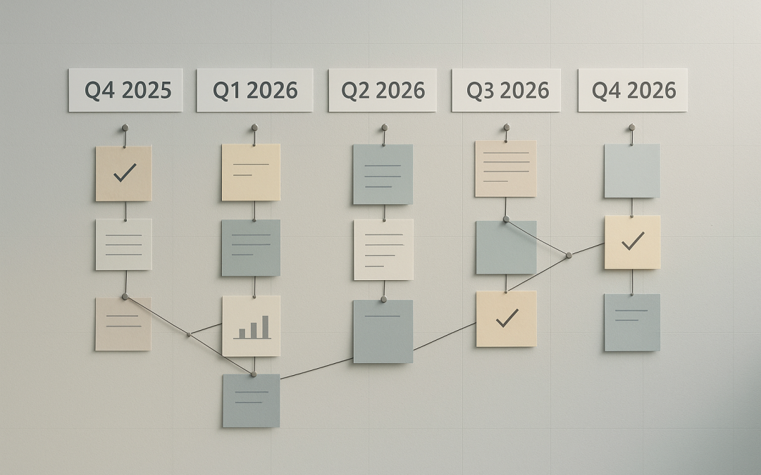
This page records work to be completed rather than retaining expired milestones or unsupported delivery promises.
Documentation
Align the current formulation, area-kernel article, notation, historical methods, and references. Consolidate duplicate content and preserve versions.
Implementation
Trace dependencies in every interactive tool. Specify which operations construct geometry, evaluate measures, compute comparison references, and draw the visualisation.
Verification
Review domains, normalisations, error proofs, rounding, cancellation, and stopping conditions. Validate general shapes and three-dimensional methods independently.
Benchmarks and Releases
Publish actual scripts, datasets, environments, licences, and measured results. Assess equal-accuracy performance before reporting a speed advantage.
Publication
List manuscripts and releases with verified status and persistent links. No release date, throughput target, or completed milestone is implied until evidence is available.
GRG integrates with structural optimization (SIMP/level set) and with machine learning for parameter calibration. Angles are measured in turns with dyadic step Δu = 2^{-n} on the full turn; a quarter has M = 2^{\,n-2} steps. Formulas remain π-free at finite resolution.
$$
n \in \mathbb{N}_{\ge 0},\qquad \Delta u = 2^{-n},\qquad M = 2^{\,n-2}\ \text{(steps per quarter)}.
$$
Topology Optimization Bridge
We expose GRG’s radial density as design variables for SIMP/level-set frameworks. Let x denote per-sector densities, mapped from radial weights:
By parameterizing x via GRG weights, the optimizer searches a low-dimensional, center-seeded space that preserves radial structure while meeting volume and stiffness targets.
Level-Set Coupling
Alternatively, drive a level-set ϕ by GRG fields: initialize ϕ from radial strips and evolve with curvature-regularized motion under structural sensitivities. GRG provides stable seeding and symmetric updates across quarters.
ML-Assisted Calibration
Given exemplars (e.g., bones, shells, corals), regress GRG parameters θ to match silhouettes or performance. Use mixed geometric + physical loss:
Radial seed & step: pick n so Δu=2^{-n}; choose rule for chords/strips (midpoint, averaged, Δx trapezoidal).
Design variables: set θ for w(u) or direct densities x(u_k).
Solver coupling: run SIMP/level-set; back-propagate sensitivities to θ.
Calibration (optional): fit θ to exemplars using the mixed loss.
Export: reconstruct full shape from quarter; output polylines/meshes.
Safety & Regularization
Step cap: enforce a minimum Δu_{\min} to prevent local collapse.
Curvature damping: penalize large changes of w(u) across adjacent sectors.
Volume guard: soft penalty if \sum x_i drifts from target fraction \bar v.
Interoperability
Inputs: seed, n, rule, parameters θ or densities x.
Outputs: perimeter P, area A, nodes/strips, optional field samples.
Formats:.OBJ polylines, .STEP (via downstream CAD), JSON config for reproducibility.
Defaults
Rule: chord — midpoint for perimeter; Δx trapezoidal for area.
n: start with n=10 (Δu=2^{-10}) and refine dyadically.
ML loss: set \lambda_{\text{geom}}=1, \lambda_{\text{phys}}=0.3, \lambda_{\text{reg}}=10^{-3} as safe starters.
Flow (left→right): GRG parameters → SIMP / Level-set solver → Performance metrics → Exports.
Dashed arc: feedback of sensitivities/gradients back to GRG (or to the ML regressor for calibration).
To provide the best experiences, we use technologies like cookies to store and/or access device information. Consenting to these technologies will allow us to process data such as browsing behavior or unique IDs on this site. Not consenting or withdrawing consent, may adversely affect certain features and functions.
Functional
Always active
The technical storage or access is strictly necessary for the legitimate purpose of enabling the use of a specific service explicitly requested by the subscriber or user, or for the sole purpose of carrying out the transmission of a communication over an electronic communications network.
Preferences
The technical storage or access is necessary for the legitimate purpose of storing preferences that are not requested by the subscriber or user.
Statistics
The technical storage or access that is used exclusively for statistical purposes.The technical storage or access that is used exclusively for anonymous statistical purposes. Without a subpoena, voluntary compliance on the part of your Internet Service Provider, or additional records from a third party, information stored or retrieved for this purpose alone cannot usually be used to identify you.
Marketing
The technical storage or access is required to create user profiles to send advertising, or to track the user on a website or across several websites for similar marketing purposes.