Concrete examples (GRG)
Here is how the value improves as you raise N (rounded):
- N = 16 → πN ≈ 3.140331156954753 (error ≈ 1.261×10⁻³)
- N = 128 → πN ≈ 3.141572940367091 (error ≈ 1.971×10⁻⁵)
- N = 1024 → πN ≈ 3.141592345570118 (error ≈ 3.080×10⁻⁷)
These numbers come straight from the turn-based chord-sum formula (angles in turns \(u\in[0,1)\) with \(s(u):=\sin(2\pi u)\)):
$$
\pi_N \;=\; 4N\,s\!\Big(\tfrac{1}{8N}\Big),
\qquad
\pi - \pi_N \;\approx\; \frac{\pi^3}{96\,N^2}.
$$
Tip: use powers of two for N (16, 32, 64, …) for cleaner Δ-tests and steadier convergence; if verified digits stop increasing when doubling N, raise working precision.
How other methods reach π (in plain words)
Long alternating sums (Gregory–Leibniz)
This is the famous series \( \pi/4 = 1 - 1/3 + 1/5 - 1/7 + \dots \).
After \(n\) terms, the error in \( \pi \) is about \( \frac{4}{2n+1} \approx \frac{2}{n} \).
It’s beautiful but very slow: ~10,000 terms give ≈4 correct decimals; ~1,000,000 terms ≈6 decimals. A mountain of fractions.
Nilakantha’s refinement
Nilakantha’s series \( \pi = 3 + \frac{4}{2\cdot3\cdot4} - \frac{4}{4\cdot5\cdot6} + \frac{4}{6\cdot7\cdot8} - \dots \) converges much faster: the error shrinks like \(1/n^2\).
Ten terms already land close; one hundred or one thousand terms push several more digits — still, you juggle many fractions.
Machin-like formulas (arctangents)
Here \( \pi \) is a combination of arctangents, e.g. \( \pi = 16\arctan(1/5) - 4\arctan(1/239) \).
The arctan series converges fast because powers \(1/5^{\,2k+1}\) and \(1/239^{\,2k+1}\) drop quickly.
With just a handful of terms you already see many correct digits.
Ramanujan, Chudnovsky & co.
“Rocket” series: each term yields many digits (≈8 per term for several Ramanujan formulas, ≈14 per term for Chudnovsky).
They power modern record computations — superb for huge digit counts, but conceptually heavier than turning a single \(N\).
AGM (Salamin–Brent) and Borwein algorithms
Iterative methods with quadratic (or higher) convergence: each step roughly multiplies the correct digits.
A dozen iterations already exceeds everyday needs — fantastic speed, less “from-the-inside” geometry.
Monte Carlo & Buffon’s needle
Random points/needles relate probabilities to \( \pi \).
Charming and educational, but accuracy grows like \(1/\sqrt{T}\) (here \(T\) = trials): even millions of trials yield only a few decimals.
Why GRG feels intellectually simple
GRG is not about naming \( \pi \); it is about holding the circle.
You dial only one parameter, \(N\), and everything else follows.
The value increases from below (no overshoot), and its error is easy to estimate.
If you truly need \( \pi \), this is the most direct, inside-out way I know — increasing a single internal factor means the computation belongs to the circle, not to an external \( \pi \).
Honest side-by-side (objective)
- What you increase — GRG: just N. Archimedean polygons: sides m (inside/outside). Gregory–Leibniz / Nilakantha: number of terms. Machin / Ramanujan / Chudnovsky: number of series terms. AGM / Borwein: iteration count.
- Speed of accuracy — GRG: error ≈ \(C/N^2\) (predictable, monotone). Gregory–Leibniz: \(O(1/n)\) (very slow). Nilakantha: \(O(1/n^2)\). Machin: fast; Ramanujan / Chudnovsky: very fast (many digits per term). AGM / Borwein: digits multiply each step.
- When to use — GRG: concept, clarity, control “from the inside”, and up to many digits without extra machinery. For records or industrial-scale digits, AGM / Borwein / Chudnovsky win on raw speed.